How to autocomplete when typing in Excel drop down list?
For a data validation drop-down list with many items, you need to scroll up and down in the list to find the one you need or type the whole word into the list box correctly. Is there any way to make the drop-down list auto-complete when typing the corresponding characters? This would help people work more efficiently in worksheets with drop-down lists in cells. This tutorial provides two methods to help you achieve it.

Make drop down lists autocomplete with VBA code
Easily make drop-down lists autocomplete in 2 seconds
More tutorials for drop down list...
Make drop down lists autocomplete with VBA code
Please do as follows to make a drop down list autocomplete after typing corresponding letters in the cell.
Firstly, you need to insert a combo box into the worksheet and change its properties.
- Open the worksheet that contains the drop down list cells you want to make them autocomplete.
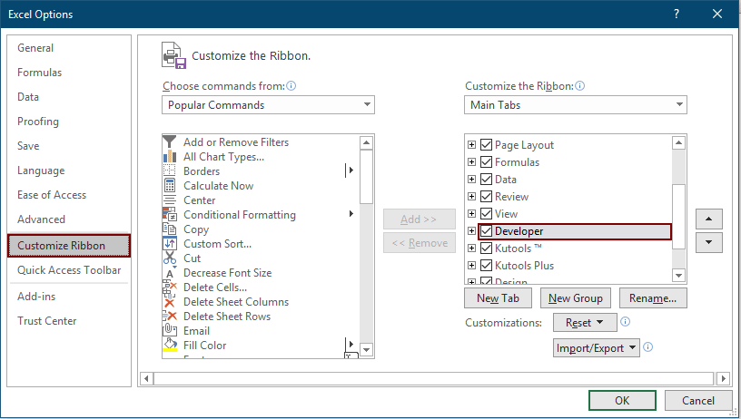
- Before inserting a Combo box, you need to add the Developer tab to the Excel ribbon. If the Developer tab is showing on your ribbon, shift to step 3. Otherwise, do as follows to get the Develper tab show up in the ribbon: Click "File" > "Options" to open the "Options" window. In this "Excel Options" window, click "Customize Ribbon" in the left pane, check the "Developer" box, and then click the "OK" button. See screenshot:
- Click "Developer" > "Insert" > "Combo Box (ActiveX Control)".

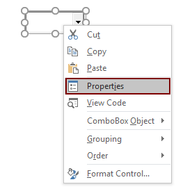
- Draw a combo box in current worksheet. Right click it and then select "Properties" from the right-clicking menu.
- In the "Properties" dialog box, please replace the original text in the "(Name)" field with "TempCombo."

- Turn off the "Design Mode" by clicking "Developer" > "Design Mode."


Then, apply the below VBA code
- Right click on current sheet tab and click "View Code" from the context menu. See screenshot:

- In the opening "Microsoft Visual Basic for Applications" window, please copy and paste the below VBA code into the worksheet’s Code window.
VBA code: Autocomplete when typing in drop down list
Private Sub Worksheet_SelectionChange(ByVal Target As Range)
'Update by Extendoffice: 2020/01/16
    Dim xCombox As OLEObject
    Dim xStr As String
    Dim xWs As Worksheet
    Dim xArr

    Set xWs = Application.ActiveSheet
    On Error Resume Next
    Set xCombox = xWs.OLEObjects("TempCombo")
    With xCombox
        .ListFillRange = ""
        .LinkedCell = ""
        .Visible = False
    End With
    If Target.Validation.Type = 3 Then
        Target.Validation.InCellDropdown = False
        Cancel = True
        xStr = Target.Validation.Formula1
        xStr = Right(xStr, Len(xStr) - 1)
        If xStr = "" Then Exit Sub
        With xCombox
            .Visible = True
            .Left = Target.Left
            .Top = Target.Top
            .Width = Target.Width + 5
            .Height = Target.Height + 5
            .ListFillRange = xStr
            If .ListFillRange = "" Then
                xArr = Split(xStr, ",")
                Me.TempCombo.List = xArr
            End If
            .LinkedCell = Target.Address
        End With
        xCombox.Activate
        Me.TempCombo.DropDown
    End If
End Sub
Private Sub TempCombo_KeyDown(ByVal KeyCode As MSForms.ReturnInteger, ByVal Shift As Integer)
    Select Case KeyCode
        Case 9
            Application.ActiveCell.Offset(0, 1).Activate
        Case 13
            Application.ActiveCell.Offset(1, 0).Activate
    End Select
End Sub
- Press "Alt + Q" keys simultaneously to close the Microsoft Visual Basic Applications window.


From now on, when click on a drop down list cell, the drop down list will prompt automatically. You can start to type in the letter to make the corresponding item complete automatically in selected cell. See screenshot:
Easily make drop-down list autocomplete in 2 seconds
For most Excel users, the above VBA method is hard to master. But with the "Searchable Drop-down List" feature of Kutools for Excel, you can easily enable autocomplete for data validation drop-down lists in a specified range in just 2 seconds. What’s more, this feature is available for all Excel versions.
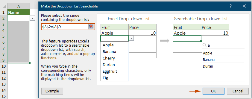
- To enable autocomplete in your dropdown lists, first select the range with the dropdowns. Then, navigate to the "Kutools" tab, choose "Drop-down List" > "Make Drop-down List Searchable, Auto-popup."
- In the "Make the Drop-down List Searchable" dialog box, click the "OK" button to save the setting.
Result
Once the configuration is complete, clicking on a drop-down list cell within the specified range will bring up a list box. When entering characters, as long as one item matches exactly, the entire word is immediately highlighted in the list box and can be populated into the drop-down list cell simply by pressing the Enter key.

Related articles:
How to create drop down list with multiple checkboxes in Excel?
Many Excel users tend to create drop down list with multiple checkboxes in order to select multiple items from the list per time. Actually, you can’t create a list with multiple checkboxes with Data Validation. In this tutorial, we are going to show you two methods to create drop down list with multiple checkboxes in Excel. This tutorial provides the method to solve the problem.
Create drop down list from another workbook in Excel
It is quite easy to create a data validation drop down list among worksheets within a workbook. But if the list data you need for the data validation locates in another workbook, what would you do? In this tutorial, you will learn how to create a drop fown list from another workbook in Excel in details.
Create a searchable drop down list in Excel
For a drop down list with numerous values, finding a proper one is not an easy work. Previously we have introduced a method of auto completing drop down list when enter the first letter into the drop down box. Besides the autocomplete function, you can also make the drop down list searchable for enhancing the working efficiency in finding proper values in the drop down list. For making drop down list searchable, try the method in this tutorial.
Auto populate other cells when selecting values in Excel drop down list
Let’s say you have created a drop down list based on the values in cell range B8:B14. When you selecting any value in the drop down list, you want the corresponding values in cell range C8:C14 be automatically populated in a selected cell. For solving the problem, the methods in this tutorial will do you a favor.
Best Office Productivity Tools
Supercharge Your Excel Skills with Kutools for Excel, and Experience Efficiency Like Never Before. Kutools for Excel Offers Over 300 Advanced Features to Boost Productivity and Save Time. Click Here to Get The Feature You Need The Most...
Office Tab Brings Tabbed interface to Office, and Make Your Work Much Easier
- Enable tabbed editing and reading in Word, Excel, PowerPoint, Publisher, Access, Visio and Project.
- Open and create multiple documents in new tabs of the same window, rather than in new windows.
- Increases your productivity by 50%, and reduces hundreds of mouse clicks for you every day!
All Kutools add-ins. One installer
Kutools for Office suite bundles add-ins for Excel, Word, Outlook & PowerPoint plus Office Tab Pro, which is ideal for teams working across Office apps.
- All-in-one suite — Excel, Word, Outlook & PowerPoint add-ins + Office Tab Pro
- One installer, one license — set up in minutes (MSI-ready)
- Works better together — streamlined productivity across Office apps
- 30-day full-featured trial — no registration, no credit card
- Best value — save vs buying individual add-in