Как да създадете падащ списък с множество квадратчета за отметка в Excel?

Много потребители на Excel са склонни да създават падащ списък с множество квадратчета за отметка, за да избират няколко елемента от списъка наведнъж. Всъщност не можете да създадете списък с множество квадратчета за отметка с валидиране на данни. В този урок ще ви покажем два метода за създаване на падащ списък с множество квадратчета за отметка в Excel.

Използвайте List Box, за да създадете падащ списък с множество квадратчета за отметка
О: Създайте списъчно поле с изходни данни
B: Назовете клетката, в която ще намерите избраните елементи
C: Вмъкнете фигура, за да помогнете за извеждането на избраните елементи
Лесно създайте падащ списък с квадратчета за отметка с невероятен инструмент
Още уроци за падащия списък...

Използвайте List Box, за да създадете падащ списък с множество квадратчета за отметка

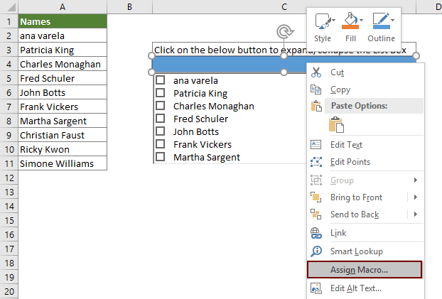
Както е показано на екранната снимка по-долу, в текущия работен лист всички имена в диапазон A2:A11 ще бъдат изходните данни на списъчното поле. Щракването върху бутона в клетка C4 може да изведе избраните елементи и всички избрани елементи в списъчното поле ще бъдат показани в клетка E4. За да постигнете това, моля, направете следното.

A. Създайте списъчно поле с изходни данни

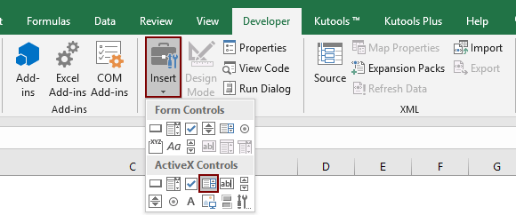
1. кликване Софтуерен Инженер > Поставете > Списъчно поле (Active X Control). Вижте екранна снимка:

2. Начертайте списъчно поле в текущия работен лист, щракнете с десния бутон върху него и след това изберете Имоти от менюто с десен бутон.

3. В Имоти диалогов прозорец, трябва да конфигурирате както следва.

• 3.1 В ListFillRange въведете диапазона на източника, който ще покажете в списъка (тук въвеждам диапазон A2: A11);
• 3.2 В ListStyle , изберете 1 - fmList StyleOption;
• 3.3 В Групов , изберете 1 – fmMultiSelectMulti;
• 3.4 Затворете Имоти диалогов прозорец. Вижте екранна снимка:

B: Назовете клетката, в която ще намерите избраните елементи

Ако трябва да изведете всички избрани елементи в определена клетка като E4, моля, направете следното.

1. Изберете клетка E4, въведете ListBoxOutput в Име Box и натиснете бутона Въведете ключ.

C. Вмъкнете фигура, за да помогнете за извеждането на избраните елементи

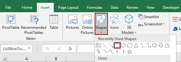
1. кликване Поставете > Фигури > Правоъгълник. Вижте екранна снимка:

2. Начертайте правоъгълник в работния си лист (тук рисувам правоъгълника в клетка C4). След това щракнете с десния бутон върху правоъгълника и изберете Присвояване на макрос от менюто с десен бутон.

3. В Присвояване на макрос кликнете върху НОВ бутон.

4. В откриването Microsoft Visual Basic за приложения прозорец, моля, заменете оригиналния код в Модули прозорец със следния VBA код.

VBA код: Създайте списък с множество квадратчета за отметка

Sub Rectangle1_Click()
'Updated by Extendoffice 20200730
Dim xSelShp As Shape, xSelLst As Variant, I, J As Integer
Dim xV As String
Set xSelShp = ActiveSheet.Shapes(Application.Caller)
Set xLstBox = ActiveSheet.ListBox1
If xLstBox.Visible = False Then
    xLstBox.Visible = True
    xSelShp.TextFrame2.TextRange.Characters.Text = "Pickup Options"
    xStr = ""
    xStr = Range("ListBoxOutput").Value
    
    If xStr <> "" Then
         xArr = Split(xStr, ";")
    For I = xLstBox.ListCount - 1 To 0 Step -1
        xV = xLstBox.List(I)
        For J = 0 To UBound(xArr)
            If xArr(J) = xV Then
              xLstBox.Selected(I) = True
              Exit For
            End If
        Next
    Next I
    End If
Else
    xLstBox.Visible = False
    xSelShp.TextFrame2.TextRange.Characters.Text = "Select Options"
    For I = xLstBox.ListCount - 1 To 0 Step -1
        If xLstBox.Selected(I) = True Then
        xSelLst = xLstBox.List(I) & ";" & xSelLst
        End If
    Next I
    If xSelLst <> "" Then
        Range("ListBoxOutput") = Mid(xSelLst, 1, Len(xSelLst) - 1)
    Else
        Range("ListBoxOutput") = ""
    End If
End If
End Sub

Забележка: в кода, Правоъгълник1 е името на формата; ListBox1 е името на списъчната кутия; Изберете Опции намлява Опции за получаване са показаните текстове на формата; и на ListBoxOutput е името на диапазона на изходната клетка. Можете да ги промените според вашите нужди.

5. Натиснете Друг + Q клавиши едновременно, за да затворите Microsoft Visual Basic за приложения прозорец.

6. Щракнете върху бутона с правоъгълник, за да сгънете или разширите списъка. Когато списъчното поле се разширява, маркирайте елементите в списъчното поле и след това щракнете върху правоъгълника отново, за да изведете всички избрани елементи в клетка E4. Вижте демонстрацията по-долу:

7. След това запазете работната книга като Excel MacroEnable Workbook за повторно използване на кода в бъдеще.

Създайте падащ списък с квадратчета за отметка с невероятен инструмент

Освен горната демонстрация, ние предоставяме и ръководство стъпка по стъпка, за да демонстрираме как да приложите тази функция за постигане на тази задача. Моля, направете следното.

1. Отворете работния лист, в който сте задали падащия списък за валидиране на данни, щракнете Kutools > Падащ списък > Падащ списък с квадратчета за отметка > Настройки. Вижте екранна снимка:

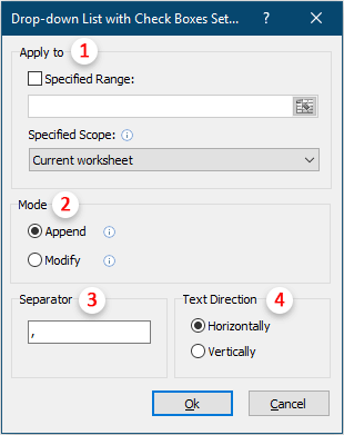
2. В Падащ списък с настройки на квадратчета за отметка диалогов прозорец, моля, конфигурирайте както следва.

• 2.1) В Нанесете раздел, посочете обхвата на прилагане, където ще създадете квадратчета за отметка за елементи в падащия списък. Можете да посочите a определен диапазон, текущ работен лист, текуща работна книга or всички отворени работни книги въз основа на вашите нужди.
• 2.2) В вид раздел, изберете стил, който искате да изведете избраните елементи;
• Тук взема Промяна опция като пример, ако изберете това, стойността на клетката ще се промени въз основа на избраните елементи.
• 2.3) В Сепаратор поле, въведете разделител, който ще използвате, за да разделите множеството елементи;
• 2.4) В Посока на текста раздел, изберете посока на текста въз основа на вашите нужди;
• 2.5) Щракнете върху OK бутон.

3. Последната стъпка, щракнете Kutools > Падащ списък > Падащ списък с квадратчета за отметка > Активирайте падащия списък с квадратчета за отметка за да активирате тази функция.

Отсега нататък, когато щракнете върху клетките с падащ списък в определен обхват, ще се появи списъчно поле, моля, изберете елементи, като поставите отметка в квадратчетата, за да ги изведете в клетка, както е показано в демонстрацията по-долу (Вземете режима на промяна като пример ).

За повече подробности относно тази функция, моля посетете тук.

Още по темата:

Най-добрите инструменти за продуктивност в офиса

🤖	Kutools AI помощник: Революционизирайте анализа на данни въз основа на: Интелигентно изпълнение   |  Генериране на код  |  Създаване на персонализирани формули  |  Анализирайте данни и генерирайте диаграми  |  Извикване на функциите на Kutools...
	Популярни функции: Намерете, маркирайте или идентифицирайте дубликати   |  Изтриване на празни редове   |  Комбинирайте колони или клетки без загуба на данни   |   Кръг без формула ...
	Супер търсене: VLookup с множество критерии  |   VLookup с множество стойности  |   VLookup в няколко листа   |   Размито търсене ....
	Разширен падащ списък: Бързо създаване на падащ списък   |  Зависим падащ списък   |  Падащ списък с множество избори ....
	Мениджър на колони: Добавете конкретен брой колони  |  Преместване на колони  |  Превключване на състоянието на видимост на скритите колони  |  Сравнете диапазони и колони ...
	Препоръчани функции: Мрежов фокус   |  Изглед на дизайна   |   Голям формула бар   |  Мениджър на работни книги и листове   |  Библиотека с ресурси (Автоматичен текст)   |  Избор на дата   |  Комбинирайте работни листове   |  Шифроване/декриптиране на клетки   |  Изпращайте имейли по списък   |  Супер филтър   |   Специален филтър (филтър получер/курсив/зачертано...) ...
	Топ 15 комплекта инструменти:  12 Текст Инструменти (добавяне на текст, Премахване на символи, ...)   |   50 + Графика Видове (диаграма на Гант, ...)   |   40+ Практичен формули (Изчислете възрастта въз основа на рождения ден, ...)   |   19 вмъкване Инструменти (Въведете QR код, Вмъкване на картина от пътя, ...)   |   12 Конверсия Инструменти (Числа към думи, Валутен обмен, ...)   |   7 Обединяване и разделяне Инструменти (Разширено комбиниране на редове, Разделени клетки, ...)   |   ... и още

Усъвършенствайте уменията си за Excel с Kutools за Excel и изпитайте ефективност, както никога досега. Kutools за Excel предлага над 300 разширени функции за повишаване на производителността и спестяване на време.  Щракнете тук, за да получите функцията, от която се нуждаете най-много...

Прочети повече ... Безплатно сваляне...

---

Раздел Office Внася интерфейс с раздели в Office и прави работата ви много по-лесна

• Разрешете редактиране и четене с раздели в Word, Excel, PowerPoint, Publisher, Access, Visio и Project.
• Отваряйте и създавайте множество документи в нови раздели на един и същ прозорец, а не в нови прозорци.
• Увеличава вашата производителност с 50% и намалява стотици кликвания на мишката за вас всеки ден!

Прочети повече ... Безплатно сваляне...