Прескочи на основното съдържание

Как да условно форматиране въз основа на друг лист в Google лист?

Автор: Xiaoyang Последна промяна: 2022-07-25

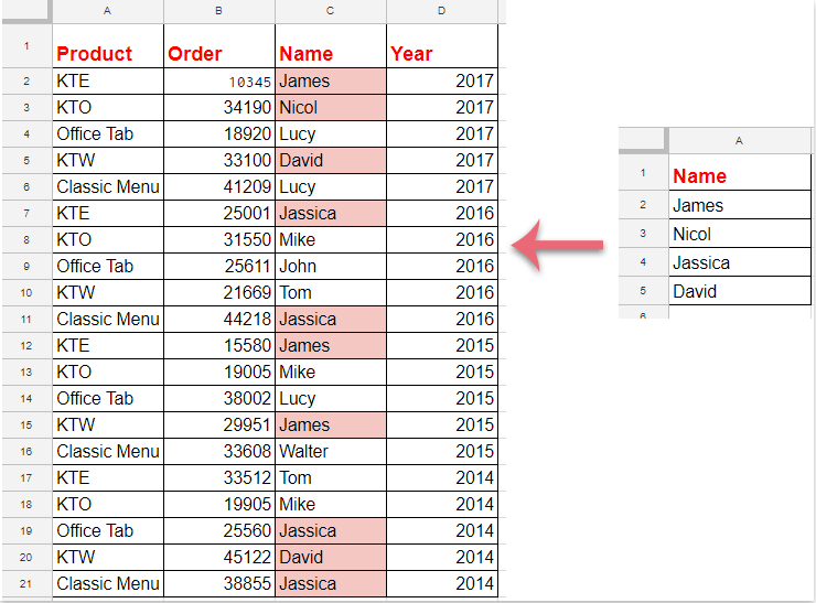
Ако искате да приложите условното форматиране, за да маркирате клетки въз основа на списък с данни от друг лист, както е показано на следващата екранна снимка в листа на Google, имате ли лесни и добри методи за решаването му?

Условно форматиране за маркиране на клетки въз основа на списък от друг лист в Google Таблици


Условно форматиране за маркиране на клетки въз основа на списък от друг лист в Google Таблици


Моля, изпълнете следните стъпки, за да завършите тази работа:

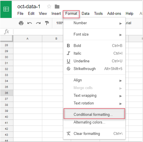
1. Щракнете формат > Условно форматиране, вижте екранна снимка:

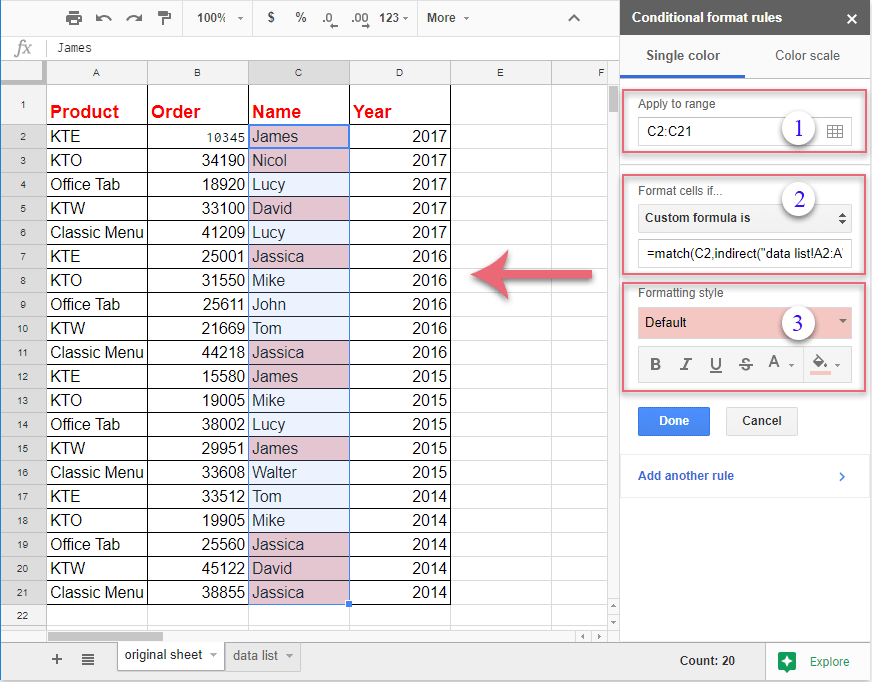
2. В Правила за условен формат прозорец, моля, извършете следните операции:

(1.) Щракнете бутон, за да изберете данните в колоната, които искате да маркирате;

(2.) В Форматиране на клетки, ако падащ списък, моля изберете Персонализираната формула е опция и след това въведете тази формула: =съвпадение(C2,indirect("списък с данни!A2:A"),0) в текстовото поле;

(3.) След това изберете едно форматиране от Стил на форматиране както ви е нужно.

Забележка: В горната формула: C2 е първата клетка от данните в колоната, която искате да маркирате, и списък с данни!A2:A е името на листа и диапазонът от клетки на списъка, който съдържа критериите, въз основа на които искате да маркирате клетките.

3. И всички съвпадащи клетки въз основа на клетките от списъка са маркирани наведнъж, тогава трябва да щракнете върху Направен за да затворите Правила за условен формат прозорец, както ви трябва.


Най-добрите инструменти за продуктивност в офиса

🤖 Kutools AI помощник: Революционизирайте анализа на данни въз основа на: Интелигентно изпълнение   |  Генериране на код  |  Създаване на персонализирани формули  |  Анализирайте данни и генерирайте диаграми  |  Извикване на функциите на Kutools...
Популярни функции: Намерете, маркирайте или идентифицирайте дубликати   |  Изтриване на празни редове   |  Комбинирайте колони или клетки без загуба на данни   |   Кръг без формула ...
Супер търсене: VLookup с множество критерии    VLookup с множество стойности  |   VLookup в няколко листа   |   Размито търсене ....
Разширен падащ списък: Бързо създаване на падащ списък   |  Зависим падащ списък   |  Падащ списък с множество избори ....
Мениджър на колони: Добавете конкретен брой колони  |  Преместване на колони  |  Превключване на състоянието на видимост на скритите колони  |  Сравнете диапазони и колони ...
Препоръчани функции: Мрежов фокус   |  Изглед на дизайна   |   Голям формула бар    Мениджър на работни книги и листове   |  Библиотека с ресурси (Автоматичен текст)   |  Избор на дата   |  Комбинирайте работни листове   |  Шифроване/декриптиране на клетки    Изпращайте имейли по списък   |  Супер филтър   |   Специален филтър (филтър получер/курсив/зачертано...) ...
Топ 15 комплекта инструменти12 Текст Инструменти (добавяне на текст, Премахване на символи, ...)   |   50 + Графика Видове (диаграма на Гант, ...)   |   40+ Практичен формули (Изчислете възрастта въз основа на рождения ден, ...)   |   19 вмъкване Инструменти (Въведете QR код, Вмъкване на картина от пътя, ...)   |   12 Конверсия Инструменти (Числа към думи, Валутен обмен, ...)   |   7 Обединяване и разделяне Инструменти (Разширено комбиниране на редове, Разделени клетки, ...)   |   ... и още

Усъвършенствайте уменията си за Excel с Kutools за Excel и изпитайте ефективност, както никога досега. Kutools за Excel предлага над 300 разширени функции за повишаване на производителността и спестяване на време.  Щракнете тук, за да получите функцията, от която се нуждаете най-много...

Описание


Раздел Office Внася интерфейс с раздели в Office и прави работата ви много по-лесна

  • Разрешете редактиране и четене с раздели в Word, Excel, PowerPoint, Publisher, Access, Visio и Project.
  • Отваряйте и създавайте множество документи в нови раздели на един и същ прозорец, а не в нови прозорци.
  • Увеличава вашата производителност с 50% и намалява стотици кликвания на мишката за вас всеки ден!


Comments (27)
Rated 5 out of 5 · 2 ratings
This comment was minimized by the moderator on the site
Hi! skyyang ! Thank you, =match(C2,indirect("data list!A2:A"),0) works for me.

But I would like to format more than one column, so column A in sheet a is checked against column B in sheet b , and so.
There are so many columns so I can not apply one format per column, but a whole conditional format for the whole sheet.


How should I modify the range and the formula?

Thanks!
This comment was minimized by the moderator on the site
What if the cell values you're trying to match are hyperlinks?
Rated 5 out of 5
This comment was minimized by the moderator on the site
Pardon, il fallait lire =A1<>INDIRECT("PreviousVersion!"& CHAR (COLUMN () + 64) & ROW ()) ...
This comment was minimized by the moderator on the site
Bonjour,
J'ai une autre question du même type au sujet d'un formatage conditionnel qui fonctionne sur Excel mais que je n'arrive pas à porter sur Google Sheet :
L'idée est de comparer 2 versions d'une même feuille que l'on stock à l'aide de 2 onglets (2 feuilles du même workbook)

La formule est la suivante : =A1<>'previousVersion'!A1 avec un formatage fond jaune pour mettre en évidence les changements sur toute la feuille car l'idée est d'appliquer ce
formatage conditionnel sur toutes les cellules de la feuille ($A$1:$V:1000)

Sur Google sheet cette formule m'est interdite et si je passe par un "indirect("previousVersion!A1"), je perds le coté dynamique sur le "A1" de la feuille precious version
Si j'essaye =A1<>indirect("previousVersion!"&A1) j'ai une erreur car c'est la valeur de A1 qui est interprétée et concaténée avec "previousVersion!"

Si j'essaye la formule =C3<>INDIRECT("PreviousVersion!"& CHAR (COLUMN () + 64) & ROW ()) cela ne fonctionne pas non plus....

Si vous avez une solution...
Merci d'avance
This comment was minimized by the moderator on the site
Bonjour,
Dans Feuille google je cherche la formule suivante
Si dans la cel A1 = text alors dans la Cel B1 ecire telle valeur ou texte automatiquement
Merci d avance pour votre aide
This comment was minimized by the moderator on the site
What if it's not an exact match but contains the reference data.
This comment was minimized by the moderator on the site
Hello, ashley
To solve your problem, please apply the below formula:
=REGEXMATCH(C2:C21,INDIRECT("Sheet2!$A$2"))

Please try, hope it can help you!
This comment was minimized by the moderator on the site
What happens if the data in my list is in more than one column? When I try to use datalist!A2:M or datalist!A:M or datalist!A2:M17 none of those work.
This comment was minimized by the moderator on the site
I have even tried naming the specific range I want to refer to and using that in the formula, no luck.
This comment was minimized by the moderator on the site
How to highlight the entire row data with conditional formatting using other sub-sheet
This comment was minimized by the moderator on the site
Hello, Ranganath
To highlight the entire row based on the data list, please do as this:
1. In the Apply to range box, select the whole sheet;
2. Apply this formula: =match($C2,indirect("datalist!A2:A"),0) into the Custom formula is textbox.
Please try, hope it can help you!

https://www.extendoffice.com/images/stories/comments/comment-skyyang/doc-highlight-entire-row.png
This comment was minimized by the moderator on the site
Hey, Thanks for replying. I have tried the formula but its not working.
Rated 5 out of 5
This comment was minimized by the moderator on the site
Hi,
Have you modified the sheet name and cell reference to your own data?
$C2 is the first cell of the column data that you want to highlight, and the datalist!A2:A is another sheet name and list range which contains the criteria you want to highlight the cells based on.
Please check them, thank you!
This comment was minimized by the moderator on the site
This doesn't work for me. I have triple checked everything.

Apply to range: K1:K2158

=match(K2,indirect("TorontoCitys!A1:A"),0)

It highlights random other city names, not in the TorontoCity's list.

K2 (is my main sheet and the starting column cell of the column I want to be affected.
TorontoCitys (is the name of the sheet)
A1 is the start of the column of the list of city names.
A is the column.

Could be that my punctuation's are incorrect?

Thanks in advance.
This comment was minimized by the moderator on the site
Hello friend,

Glad to help. Your formula is correct, please don't worry. The problem is the range you apply to. It shouldn't be K1:K2158, but K2:K2158.

Please see the screenshots. The example is simple but enough to explain the problem.

The correct "Apply to Range" is A2:A20. And the correct formula is =match(A2,indirect("TorontoCitys!A1:A"),0). Then correct cities can be highlighted. Please see screenshot 2.
But if I change the "Apply to Range" to A1:A20, the wrong city name is highlighted. Please see screenshot 3.

So please change your "Apply to Range" from K1:K2158 to K2:K2158. The problem should be solved. Looking forward to your reply.

Sincerely,
Mandy
This comment was minimized by the moderator on the site
how do you do this but with the entire row highlighted
There are no comments posted here yet
Load More
Please leave your comments in English
Posting as Guest
×
Rate this post:
0   Characters
Suggested Locations