Прескочи на основното съдържание

Как да дефинирам диапазон въз основа на друга стойност на клетка в Excel?

Автор: Слънце Последна промяна: 2020-06-24

Изчисляването на диапазон от стойности е лесно за повечето потребители на Excel, но опитвали ли сте някога да изчислите диапазон от стойности въз основа на числото в конкретна клетка? Например има колона със стойности в колона A и искам да изчисля броя на стойностите в колона A въз основа на стойността в B2, което означава, че ако е 4 в B2, ще осредня първите 4 стойности в колона A, както е показано на екранната снимка по-долу. Сега представям проста формула за бързо дефиниране на диапазон въз основа на друга стойност на клетка в Excel.
doc дефиниране на диапазон чрез стойност на клетка 1

Определете диапазон въз основа на стойността на клетката


стрелка син десен балон Определете диапазон въз основа на стойността на клетката

За да направите изчисление за диапазон въз основа на стойност на друга клетка, можете да използвате проста формула.

Изберете празна клетка, в която ще изведете резултата, въведете тази формула =СРЕДНО(A1:INDIRECT(CONCATENATE("A",B2))), и натиснете Въведете ключ за получаване на резултата.
doc дефиниране на диапазон чрез стойност на клетка 2

Забележка:

1. Във формулата A1 е първата клетка в колоната, която искате да изчислите, A е колоната, за която изчислявате, B2 е клетката, на базата на която изчислявате. Можете да промените тези препратки според нуждите си.

2. Ако искате да направите обобщение, можете да използвате тази формула =SUM(A1:INDIRECT(CONCATENATE("A",B2))).

3. Ако първите данни, които искате да дефинирате, не са в първия ред в Excel, например в клетка A2, можете да използвате формулата по следния начин: =СРЕДНО(A2:INDIRECT(CONCATENATE("A",RED(A2)+B2-1))).
doc дефиниране на диапазон чрез стойност на клетка 2


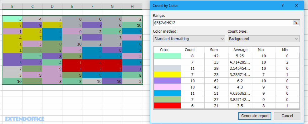
Бързо преброяване/сумиране на клетки по фон или цвят на формат в Excel

В някои случаи може да имате диапазон от клетки с множество цветове и това, което искате, е да преброите/сумирате стойности въз основа на един и същи цвят, как можете бързо да изчислите?
с Kutools за Excel's Брой по цвят, можете бързо да правите много изчисления по цвят, а също така можете да генерирате отчет за изчисления резултат.  Кликнете за безплатен пълнофункционален пробен период след 30 дни!
брой документи по цвят 1
 
Kutools за Excel: с повече от 300 удобни добавки за Excel, безплатни за изпробване без ограничение за 30 дни.

Най-добрите инструменти за продуктивност в офиса

🤖 Kutools AI помощник: Революционизирайте анализа на данни въз основа на: Интелигентно изпълнение   |  Генериране на код  |  Създаване на персонализирани формули  |  Анализирайте данни и генерирайте диаграми  |  Извикване на функциите на Kutools...
Популярни функции: Намерете, маркирайте или идентифицирайте дубликати   |  Изтриване на празни редове   |  Комбинирайте колони или клетки без загуба на данни   |   Кръг без формула ...
Супер търсене: VLookup с множество критерии    VLookup с множество стойности  |   VLookup в няколко листа   |   Размито търсене ....
Разширен падащ списък: Бързо създаване на падащ списък   |  Зависим падащ списък   |  Падащ списък с множество избори ....
Мениджър на колони: Добавете конкретен брой колони  |  Преместване на колони  |  Превключване на състоянието на видимост на скритите колони  |  Сравнете диапазони и колони ...
Препоръчани функции: Мрежов фокус   |  Изглед на дизайна   |   Голям формула бар    Мениджър на работни книги и листове   |  Библиотека с ресурси (Автоматичен текст)   |  Избор на дата   |  Комбинирайте работни листове   |  Шифроване/декриптиране на клетки    Изпращайте имейли по списък   |  Супер филтър   |   Специален филтър (филтър получер/курсив/зачертано...) ...
Топ 15 комплекта инструменти12 Текст Инструменти (добавяне на текст, Премахване на символи, ...)   |   50 + Графика Видове (диаграма на Гант, ...)   |   40+ Практичен формули (Изчислете възрастта въз основа на рождения ден, ...)   |   19 вмъкване Инструменти (Въведете QR код, Вмъкване на картина от пътя, ...)   |   12 Конверсия Инструменти (Числа към думи, Валутен обмен, ...)   |   7 Обединяване и разделяне Инструменти (Разширено комбиниране на редове, Разделени клетки, ...)   |   ... и още

Усъвършенствайте уменията си за Excel с Kutools за Excel и изпитайте ефективност, както никога досега. Kutools за Excel предлага над 300 разширени функции за повишаване на производителността и спестяване на време.  Щракнете тук, за да получите функцията, от която се нуждаете най-много...

Описание


Раздел Office Внася интерфейс с раздели в Office и прави работата ви много по-лесна

  • Разрешете редактиране и четене с раздели в Word, Excel, PowerPoint, Publisher, Access, Visio и Project.
  • Отваряйте и създавайте множество документи в нови раздели на един и същ прозорец, а не в нови прозорци.
  • Увеличава вашата производителност с 50% и намалява стотици кликвания на мишката за вас всеки ден!
Comments (21)
No ratings yet. Be the first to rate!
This comment was minimized by the moderator on the site
But If I want to sum a column range(say l7:l7800) out of the range d7:ct9000 based on the condition in column a(a7:a9000) and column b(b7:b9000). How will I do it. Please advise
This comment was minimized by the moderator on the site
Is there a way to create a dynamic ranged view, that will isolate all orders from a specific client within a list of clients? I have looked at multiple videos and none actually do what I need it to do. Is there a way to do this or would I need to pull the needed info into a controlled table and use the information from that table?
This comment was minimized by the moderator on the site
Hi, CareTaker. I do not get your question clearly. Could you describe your question or upload a file to show the quetion in details? But I recomend a utility called Data Association for you, maybe can help you, go to this web for details: https://www.extendoffice.com/product/kutools-for-excel/excel-click-cell-to-filter-based-on-another-workbook.html.
This comment was minimized by the moderator on the site
Thank you for the response, its quite the complicated thing to explain but I did manage to come right in the end using the indexing formula with the match formula as well.   =INDEX($B:$B;MATCH($C$2;$B:$B;0);):INDEX($N:$N;MATCH($C$2;$B:$B;0)+$C$3-1;)   at first it was confusing but I'm good now 
This comment was minimized by the moderator on the site
how do I update sum range by using helper cell...For example: if initial sum range is = C1 to M1, how to do change sum range if new data is up to AB1 using a helper cell, instead of changing the formula manually?
This comment was minimized by the moderator on the site
What if the rage is not column, but a row?
This comment was minimized by the moderator on the site
That's a bit trickier as I just found out. You need to use a combination of the CHAR function to convert a number to a letter, CONCAT to piece together a letter and number comprising a cell address, and the INDIRECT function to recognize strings as cell addresses.

In my example, I wrote the following expression:

=SUM(INDIRECT(CONCAT("F",ROW())):INDIRECT(CONCAT(CHAR(64+5+$B$31),ROW())))


where:
Row() is the current row
$B$31 is the cell where the # of columns to count is stored
5 is the offset for the first column to be counted

if you need to go beyond column Z, you’d need a less intuitive variant on that expression using the ADDRESS function:

=SUM(indirect(concat("F",row())):indirect(ADDRESS(row(),$B$31+5,4)))


where:
4 indicates a relative reference
This comment was minimized by the moderator on the site
Hi quick question. My formula =SUMIFS(DATA!$D$5:$D$13914,DATA!$E$5:INDIRECT(CONCATENATE("$E$",C3)),"<"&"1/1/2016") has a range that is from another tab called "DATA." I keep getting #VALUE! errors for this formula. Any suggestions? thanks!
This comment was minimized by the moderator on the site
Earlier I posted: Great formula but why does it only work when referring to the first cell. In other words, if you move the whole range down and the first cell in the range is A5 instead of A1, the formula ceases to work.
After playing with it, I figured out why the formula is not working when the starting row is not row 1. Excel interprets this as the range being A1 thru A4. If you are starting with a different row than row 1, here is how to modify the formula assuming the range now starts with A5:=MAX(A5:INDIRECT(CONCATENATE("A",ROW(A5)+B2)))
This works because the concatenation sees the row reference as fixed in the first example, but it becomes relative in the second example. Hope that helps!
Jared - You can just subtract 4 instead of adding. =MAX(A5:INDIRECT(CONCATENATE("A",ROW(A5)-B2))) [Assuming you have 4 in cell B2, or you could just leave the formula as is and put -4 in cell B2.]
This comment was minimized by the moderator on the site
Hi,cathy, thanks for your supplement, I have test your formula, I think the correct formula may be =MAX(A5:INDIRECT(CONCATENATE("A",ROW(A5)+B2-1))). I have update the tutorual. Thanks again.
This comment was minimized by the moderator on the site
Great formula but why does it only work when referring to the first cell. In other words, if you move the whole range down and the first cell in the range is A6 instead of A1, the formula ceases to work. That seems strange.
This comment was minimized by the moderator on the site
What if I want to count upward from a cell rather than downward? In the above example, the formula starts with A1 and goes downward. Let's say I want a range of 4 cells, beginning with Cell A10 and going to A6. Thank you!
This comment was minimized by the moderator on the site
Jared - See my most recent post for how to solve this.
This comment was minimized by the moderator on the site
I'm having this upward problem also but unable to see your other post for the solution. Can you give me link of the post please? Many thanks!
This comment was minimized by the moderator on the site
Hi, here is a formula may help you to calcualte upward.
=AVERAGE(INDIRECT(CONCATENATE("A",COUNT(A:A)-B1+1)):INDIRECT(CONCATENATE("A",COUNT(A:A))))
A:A is the column that you want to calcualte the average values, B1 is the cell that define the range in column A to calculate.
This comment was minimized by the moderator on the site
Thanks, but may I know why need to use "-B1+1" please?
This comment was minimized by the moderator on the site
Hi, Let me take a detailed example to explain it for you. There are 10 rows in column A, I want to get the last 2 values' average, in other words, average the values in row 9 and row 10. Now B1 contains 2, =COUNT(A:A)-B1+1 will get the result 9, COUNT(A:A) will get the result 10 (the last row of the column A). Now combine other functions to averaget the values in row 9 and row 10. Hope this can help you.
This comment was minimized by the moderator on the site
Can I use this syntax while referring to a different sheet?
This comment was minimized by the moderator on the site
If you want to sum referring to a Different Shet In CONCATENATE formula write [ SHEET NAME+COLUMN+ROW]
Formula=SUM(INDIRECT(CONCATENATE("Sheet1!","D",1)):INDIRECT(CONCATENATE("Sheet1!","D",5)))
This comment was minimized by the moderator on the site
Hi, Thank you so much for your help, but I have a small problem that is I don't have just one column but several ones (about 100 columns) is there a way to change the formula to accommodate the change in columns so O can get the sum for Columns A B C and so on. thanks for your help
This comment was minimized by the moderator on the site
Thank u for your message. If you want to sum first n values across multiple continuous columns, just change A to the last column you ues. EG, sum first 5 values across column A to column D, apply this formula =SUM(A1:INDIRECT(CONCATENATE("D",F2))).
There are no comments posted here yet
Please leave your comments in English
Posting as Guest
×
Rate this post:
0   Characters
Suggested Locations