Прескочи на основното съдържание

Как да променя цвета на формата въз основа на стойността на клетката в Excel?

Автор: Xiaoyang Последна промяна: 2016-07-06

Промяната на цвета на фигурата въз основа на конкретна стойност на клетка може да бъде интересна задача в Excel, например, ако стойността на клетката в A1 е по-малка от 100, цветът на фигурата е червен, ако A1 е по-голяма от 100 и по-малка от 200, цветът на фигурата е жълт, а когато A1 е по-голям от 200, цветът на фигурата е зелен, както е показано на следната екранна снимка. За да промените цвета на фигурата въз основа на стойност на клетка, тази статия ще ви представи метод.

doc промяна на цвета на формата 1

Променете цвета на формата въз основа на стойността на клетката с VBA код


стрелка син десен балон Променете цвета на формата въз основа на стойността на клетката с VBA код

Кодът VBA по-долу може да ви помогне да промените цвета на формата въз основа на стойност на клетка, моля, направете следното:

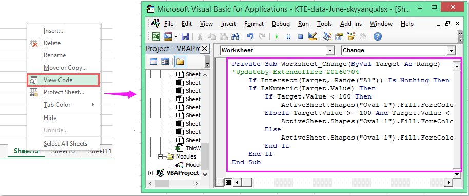
1. Щракнете с десния бутон върху раздела на листа, чийто цвят искате да промените, и след това изберете Преглед на кода от контекстното меню, в изскачащия Microsoft Visual Basic за приложения прозорец, моля, копирайте и поставете следния код в празното поле Модули прозорец.

VBA код: Променете цвета на формата въз основа на стойността на клетката:

Private Sub Worksheet_Change(ByVal Target As Range)
'Updateby Extendoffice 20160704
    If Intersect(Target, Range("A1")) Is Nothing Then Exit Sub
    If IsNumeric(Target.Value) Then
        If Target.Value < 100 Then
            ActiveSheet.Shapes("Oval 1").Fill.ForeColor.RGB = vbRed
        ElseIf Target.Value >= 100 And Target.Value < 200 Then
            ActiveSheet.Shapes("Oval 1").Fill.ForeColor.RGB = vbYellow
        Else
            ActiveSheet.Shapes("Oval 1").Fill.ForeColor.RGB = vbGreen
        End If
    End If
End Sub

doc промяна на цвета на формата 2

2. И тогава, когато въведете стойността в клетка A1, цветът на формата ще бъде променен със стойността на клетката, както сте дефинирали.

Забележка: В горния код, A1 е стойността на клетката, въз основа на която цветът на вашата фигура ще бъде променен, и Овал 1 е името на формата на вашата вмъкната форма, можете да ги промените според вашите нужди.

Най-добрите инструменти за продуктивност в офиса

🤖 Kutools AI помощник: Революционизирайте анализа на данни въз основа на: Интелигентно изпълнение   |  Генериране на код  |  Създаване на персонализирани формули  |  Анализирайте данни и генерирайте диаграми  |  Извикване на функциите на Kutools...
Популярни функции: Намерете, маркирайте или идентифицирайте дубликати   |  Изтриване на празни редове   |  Комбинирайте колони или клетки без загуба на данни   |   Кръг без формула ...
Супер търсене: VLookup с множество критерии    VLookup с множество стойности  |   VLookup в няколко листа   |   Размито търсене ....
Разширен падащ списък: Бързо създаване на падащ списък   |  Зависим падащ списък   |  Падащ списък с множество избори ....
Мениджър на колони: Добавете конкретен брой колони  |  Преместване на колони  |  Превключване на състоянието на видимост на скритите колони  |  Сравнете диапазони и колони ...
Препоръчани функции: Мрежов фокус   |  Изглед на дизайна   |   Голям формула бар    Мениджър на работни книги и листове   |  Библиотека с ресурси (Автоматичен текст)   |  Избор на дата   |  Комбинирайте работни листове   |  Шифроване/декриптиране на клетки    Изпращайте имейли по списък   |  Супер филтър   |   Специален филтър (филтър получер/курсив/зачертано...) ...
Топ 15 комплекта инструменти12 Текст Инструменти (добавяне на текст, Премахване на символи, ...)   |   50 + Графика Видове (диаграма на Гант, ...)   |   40+ Практичен формули (Изчислете възрастта въз основа на рождения ден, ...)   |   19 вмъкване Инструменти (Въведете QR код, Вмъкване на картина от пътя, ...)   |   12 Конверсия Инструменти (Числа към думи, Валутен обмен, ...)   |   7 Обединяване и разделяне Инструменти (Разширено комбиниране на редове, Разделени клетки, ...)   |   ... и още

Усъвършенствайте уменията си за Excel с Kutools за Excel и изпитайте ефективност, както никога досега. Kutools за Excel предлага над 300 разширени функции за повишаване на производителността и спестяване на време.  Щракнете тук, за да получите функцията, от която се нуждаете най-много...

Описание


Раздел Office Внася интерфейс с раздели в Office и прави работата ви много по-лесна

  • Разрешете редактиране и четене с раздели в Word, Excel, PowerPoint, Publisher, Access, Visio и Project.
  • Отваряйте и създавайте множество документи в нови раздели на един и същ прозорец, а не в нови прозорци.
  • Увеличава вашата производителност с 50% и намалява стотици кликвания на мишката за вас всеки ден!
Comments (22)
Rated 4 out of 5 · 1 ratings
This comment was minimized by the moderator on the site
how would be the VBA code to paint several autoforms according to a range of data?
the values are in column B and I have 20 autoforms.
This comment was minimized by the moderator on the site
Como faço para para variar as cores da forma se minha opções for em formato de texto, como "Sim" e "Não"?
This comment was minimized by the moderator on the site
Hello, Emilly
To solve your problem, please apply the below code:
Private Sub Worksheet_Change(ByVal Target As Range)
If Range("A1") = "Yes" Then
ActiveSheet.Shapes("Oval 1").Fill.ForeColor.RGB = vbRed
Else
If Range("A1") = "No" Then
ActiveSheet.Shapes("Oval 1").Fill.ForeColor.RGB = vbGreen
End If
End If
End Sub


Please have a try, hope it can help you!
This comment was minimized by the moderator on the site
Hi Skyyang,

I tried the original VBA code and got it to work, although it would not activate actively when the cell changed. Today the code is not working and I also tried your more simplistic code and still did not work. The only thing that changed is that I copied the worksheet which contained the code that worked. Would this then result in it not working?
This comment was minimized by the moderator on the site
Hola, excelente ejemplo.
Pero como seria si tengo una forma y quiero ir coloreado poco a poco dependiendo del valor ejemplo:
Si el valor es 50%
Seia mitad roja y mitad verde
Pero que se vaya llenando según el porcentaje vaya aumentando
Rated 4 out of 5
This comment was minimized by the moderator on the site
I am new to VBAs and am struggling with something. I need to have 9 different cells A1-A9 change the colour of 9 different objects. Objects are cubes 1-9. Just to clarify, each cell is to change just one object A1-Cube 1, etc. Red if it fails to meet the value and green if it exceeds the value. The pass/fail value can change so instead of having the value in the VBA I need it to reference cell A10 which has the pass/fail value. Any chance someone could through out a sample code for me to work with.

Thanks
This comment was minimized by the moderator on the site
Great solution! How can I do if I have more than 1 oval in the worksheet which the colors change according to the value input say in A1, B1,C1? Thanks in advance for your reply! 
This comment was minimized by the moderator on the site
Hello mnsosa,Glad to help. Please copy and paste the below VBA code into the blank Module window.
Sub TestMacro2()
Dim dblHt As Double
Dim rngC As Range
Dim lngr As Long
Dim dblMargin As Double
Dim lngSR As Long

lngSR = 2 'Row where the data starts

dblMargin = 6 ' Distance between shapes

'On Error Resume Next
ActiveSheet.Shapes.SelectAll
Selection.Delete
On Error GoTo 0


dblHt = Rows(lngSR).Height * 4

For lngr = lngSR To Cells(lngSR, "A").End(xlDown).Row
ActiveSheet.Shapes.AddShape(msoShapeOval, _
Cells(lngSR, "D").Left + ((lngr - lngSR) Mod 4) * dblHt + dblMargin, _
Cells(lngSR, "D").Top + Int((lngr - lngSR) / 4) * dblHt + dblMargin, _
dblHt - 2 * dblMargin, _
dblHt - 2 * dblMargin).Select
Selection.Name = "Round" & Cells(lngr, "A").Address
Selection.ShapeRange.TextFrame2.VerticalAnchor = msoAnchorMiddle
Selection.ShapeRange(1).TextFrame2.TextRange.Characters.Text = Cells(lngr, "A").Value
With Selection.ShapeRange(1).TextFrame2.TextRange.Characters(1, 2).ParagraphFormat
.FirstLineIndent = 0
.Alignment = msoAlignCenter
End With
With Selection.ShapeRange(1).TextFrame2.TextRange.Characters(1, 2).Font
.Bold = msoTrue
.Fill.Visible = msoTrue
.Fill.ForeColor.ObjectThemeColor = msoThemeColorText1
.Fill.ForeColor.TintAndShade = 0
.Fill.ForeColor.Brightness = 0
.Fill.Transparency = 0
.Fill.Solid
.Size = 12
End With
With Selection.ShapeRange.Fill
.Visible = msoTrue
If Cells(lngr, "A").Value > 70 Then
.ForeColor.RGB = RGB(0, 176, 80)
ElseIf Cells(lngr, "A").Value >= 40 Then
.ForeColor.RGB = RGB(255, 255, 70)
Else
.ForeColor.RGB = RGB(255, 0, 0)
End If
.Transparency = 0
.Solid
End With
Next lngr
Range("A1").Select
End Sub

After you run the VBA code above, you will see multiple shapes are generated, and the colors of these shapes are changed according to the VBA.Please see my screenshot. Hope it can help. Have a nice day.Sincerely,Mandy
This comment was minimized by the moderator on the site
¿Cómo hacemos si tenemos más de 1 Oval en la hoja de trabajo cuyos colores cambian de acuerdo con el valor ingresado, por ejemplo, en A1, B1, C1...? Mil gracias por su ayuda!

This comment was minimized by the moderator on the site
Hello María Noel,
Glad to help. Please copy and paste the below VBA code into the blank Module window.

Sub TestMacro2()
Dim dblHt As Double
Dim rngC As Range
Dim lngr As Long
Dim dblMargin As Double
Dim lngSR As Long

lngSR = 2 'Row where the data starts

dblMargin = 6 ' Distance between shapes

'On Error Resume Next
ActiveSheet.Shapes.SelectAll
Selection.Delete
On Error GoTo 0


dblHt = Rows(lngSR).Height * 4

For lngr = lngSR To Cells(lngSR, "A").End(xlDown).Row
ActiveSheet.Shapes.AddShape(msoShapeOval, _
Cells(lngSR, "D").Left + ((lngr - lngSR) Mod 4) * dblHt + dblMargin, _
Cells(lngSR, "D").Top + Int((lngr - lngSR) / 4) * dblHt + dblMargin, _
dblHt - 2 * dblMargin, _
dblHt - 2 * dblMargin).Select
Selection.Name = "Round" & Cells(lngr, "A").Address
Selection.ShapeRange.TextFrame2.VerticalAnchor = msoAnchorMiddle
Selection.ShapeRange(1).TextFrame2.TextRange.Characters.Text = Cells(lngr, "A").Value
With Selection.ShapeRange(1).TextFrame2.TextRange.Characters(1, 2).ParagraphFormat
.FirstLineIndent = 0
.Alignment = msoAlignCenter
End With
With Selection.ShapeRange(1).TextFrame2.TextRange.Characters(1, 2).Font
.Bold = msoTrue
.Fill.Visible = msoTrue
.Fill.ForeColor.ObjectThemeColor = msoThemeColorText1
.Fill.ForeColor.TintAndShade = 0
.Fill.ForeColor.Brightness = 0
.Fill.Transparency = 0
.Fill.Solid
.Size = 12
End With
With Selection.ShapeRange.Fill
.Visible = msoTrue
If Cells(lngr, "A").Value > 70 Then
.ForeColor.RGB = RGB(0, 176, 80)
ElseIf Cells(lngr, "A").Value >= 40 Then
.ForeColor.RGB = RGB(255, 255, 70)
Else
.ForeColor.RGB = RGB(255, 0, 0)
End If
.Transparency = 0
.Solid
End With
Next lngr
Range("A1").Select
End Sub

After you run the VBA code above, you will see multiple shapes are generated, and the colors of these shapes are changed according to the VBA.
Please see my screenshot. Hope it can help. Have a nice day.
Sincerely,
Mandy
This comment was minimized by the moderator on the site
Hi... excellent solution... but how do I apply it to multiple shapes based on the corresponding values of a range of cells. Many thanks in advance for your help.
This comment was minimized by the moderator on the site
Hello Ryan,
Glad to help. Please copy and paste the below VBA code into the blank Module window.

Sub TestMacro2()
Dim dblHt As Double
Dim rngC As Range
Dim lngr As Long
Dim dblMargin As Double
Dim lngSR As Long

lngSR = 2 'Row where the data starts

dblMargin = 6 ' Distance between shapes

'On Error Resume Next
ActiveSheet.Shapes.SelectAll
Selection.Delete
On Error GoTo 0


dblHt = Rows(lngSR).Height * 4

For lngr = lngSR To Cells(lngSR, "A").End(xlDown).Row
ActiveSheet.Shapes.AddShape(msoShapeOval, _
Cells(lngSR, "D").Left + ((lngr - lngSR) Mod 4) * dblHt + dblMargin, _
Cells(lngSR, "D").Top + Int((lngr - lngSR) / 4) * dblHt + dblMargin, _
dblHt - 2 * dblMargin, _
dblHt - 2 * dblMargin).Select
Selection.Name = "Round" & Cells(lngr, "A").Address
Selection.ShapeRange.TextFrame2.VerticalAnchor = msoAnchorMiddle
Selection.ShapeRange(1).TextFrame2.TextRange.Characters.Text = Cells(lngr, "A").Value
With Selection.ShapeRange(1).TextFrame2.TextRange.Characters(1, 2).ParagraphFormat
.FirstLineIndent = 0
.Alignment = msoAlignCenter
End With
With Selection.ShapeRange(1).TextFrame2.TextRange.Characters(1, 2).Font
.Bold = msoTrue
.Fill.Visible = msoTrue
.Fill.ForeColor.ObjectThemeColor = msoThemeColorText1
.Fill.ForeColor.TintAndShade = 0
.Fill.ForeColor.Brightness = 0
.Fill.Transparency = 0
.Fill.Solid
.Size = 12
End With
With Selection.ShapeRange.Fill
.Visible = msoTrue
If Cells(lngr, "A").Value > 70 Then
.ForeColor.RGB = RGB(0, 176, 80)
ElseIf Cells(lngr, "A").Value >= 40 Then
.ForeColor.RGB = RGB(255, 255, 70)
Else
.ForeColor.RGB = RGB(255, 0, 0)
End If
.Transparency = 0
.Solid
End With
Next lngr
Range("A1").Select
End Sub

After you run the VBA code above, you will see multiple shapes are generated, and the colors of these shapes are changed according to the VBA.
Please see my screenshot. Hope it can help. Have a nice day.
Sincerely,
Mandy
This comment was minimized by the moderator on the site
How do I make the private sub to read the result from the AVERAGE(C1,C5,C9) calculation?

Sub only works with numeric values; any thoughts and suggestions are greatly appreciated.
This comment was minimized by the moderator on the site
Hello Cesare,How are you? I notice that the VBA code can work with the AVERAGE(number, number...) calculation. But the trick is that every time you change the values in the calculation, you need to double-click the formula in the cell to make the VBA work again. 
For example, In cell A1, after we input the formula is =AVERAGE(C2:D3), the VBA works and changes the color of the shape accordingly. Please see screenshot 1. <span style="letter-spacing: 0.2px; color: inherit; font-family: inherit; font-style: inherit; font-variant-ligatures: inherit; font-variant-caps: inherit; font-weight: inherit;">C2:D3, the returned result in cell A1 changes, but the shape color hasn't been changed yet. In this case, we need to double click the formula in cell A1 to make the VBA work. Then the shape color will be changed accordingly. Please see screenshots 2 and 3.</span>
This comment was minimized by the moderator on the site
Thanks for this which is really useful.

I now want to use it with a pivot table on another worksheet which controls the data on the sheet with the shapes that I want to change colour. However, when I change the selection on the pivot table the data on the worksheet with the shapes is updated but the code does not run so the shapes do not change colour

If I manually change the values the code runs and the colour of the shapes is updated.

Question: what do i need to add to the code above to allow it to run automatically?
This comment was minimized by the moderator on the site
How can this be applied if you have multiple shape in the same worksheet?
This comment was minimized by the moderator on the site
Hello Yasir,
Glad to help. Please copy and paste the below VBA code into the blank Module window.

Sub TestMacro2()
Dim dblHt As Double
Dim rngC As Range
Dim lngr As Long
Dim dblMargin As Double
Dim lngSR As Long

lngSR = 2 'Row where the data starts

dblMargin = 6 ' Distance between shapes

'On Error Resume Next
ActiveSheet.Shapes.SelectAll
Selection.Delete
On Error GoTo 0


dblHt = Rows(lngSR).Height * 4

For lngr = lngSR To Cells(lngSR, "A").End(xlDown).Row
ActiveSheet.Shapes.AddShape(msoShapeOval, _
Cells(lngSR, "D").Left + ((lngr - lngSR) Mod 4) * dblHt + dblMargin, _
Cells(lngSR, "D").Top + Int((lngr - lngSR) / 4) * dblHt + dblMargin, _
dblHt - 2 * dblMargin, _
dblHt - 2 * dblMargin).Select
Selection.Name = "Round" & Cells(lngr, "A").Address
Selection.ShapeRange.TextFrame2.VerticalAnchor = msoAnchorMiddle
Selection.ShapeRange(1).TextFrame2.TextRange.Characters.Text = Cells(lngr, "A").Value
With Selection.ShapeRange(1).TextFrame2.TextRange.Characters(1, 2).ParagraphFormat
.FirstLineIndent = 0
.Alignment = msoAlignCenter
End With
With Selection.ShapeRange(1).TextFrame2.TextRange.Characters(1, 2).Font
.Bold = msoTrue
.Fill.Visible = msoTrue
.Fill.ForeColor.ObjectThemeColor = msoThemeColorText1
.Fill.ForeColor.TintAndShade = 0
.Fill.ForeColor.Brightness = 0
.Fill.Transparency = 0
.Fill.Solid
.Size = 12
End With
With Selection.ShapeRange.Fill
.Visible = msoTrue
If Cells(lngr, "A").Value > 70 Then
.ForeColor.RGB = RGB(0, 176, 80)
ElseIf Cells(lngr, "A").Value >= 40 Then
.ForeColor.RGB = RGB(255, 255, 70)
Else
.ForeColor.RGB = RGB(255, 0, 0)
End If
.Transparency = 0
.Solid
End With
Next lngr
Range("A1").Select
End Sub

After you run the VBA code above, you will see multiple shapes are generated, and the colors of these shapes are changed according to the VBA.
Please see my screenshot. Hope it can help. Have a nice day.
Sincerely,
Mandy
There are no comments posted here yet
Load More
Please leave your comments in English
Posting as Guest
×
Rate this post:
0   Characters
Suggested Locations