Прескочи на основното съдържание

Как да свържа клетки, ако същата стойност съществува в друга колона в Excel?

Автор: Силувия Последна промяна: 2023-04-23

Както е показано на екранната снимка по-долу, ако искате да свържете клетки във втората колона въз основа на същите стойности в първата колона, има няколко метода, които можете да използвате. В тази статия ще представим три начина за изпълнение на тази задача.

комбинирайте, ако е същото


Свързване на клетки, ако стойността е еднаква, с формули и филтър

Следните формули помагат за свързване на съдържанието на съответните клетки в колона въз основа на същата стойност в друга колона.

1. Изберете празна клетка освен втората колона (тук избираме клетка C2), въведете формула =АКО(A2<>A1,B2,C1 & "," & B2) в лентата с формули и след това натиснете Въведете ключ.

2. След това изберете клетка C2 и плъзнете манипулатора за попълване надолу до клетките, които трябва да свържете.

3. Въведете формула =АКО(A2<>A3,СЪЕДИНЯВАНЕ(A2,",""",C2,""""),"") в клетка D2 и плъзнете манипулатора за запълване надолу до останалите клетки.

4. Изберете клетка D1 и щракнете Дата > филтър. Вижте екранна снимка:

5. Щракнете върху падащата стрелка в клетка D1, премахнете отметката от (Празни) и след това щракнете върху OK бутон.

Можете да видите, че клетките са свързани, ако стойностите на първата колона са еднакви.

Забележка: За да използвате горните формули успешно, едни и същи стойности в колона A трябва да са непрекъснати.


Лесно свързване на клетки, ако има същата стойност с Kutools за Excel (няколко кликвания)

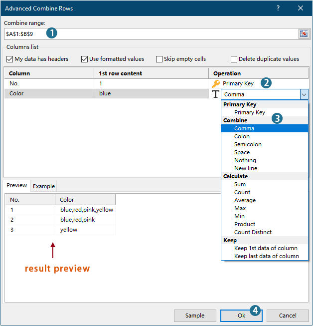
Методът, описан по-горе, изисква създаване на две помощни колони и включва множество стъпки, което може да е неудобно. Ако търсите по-прост начин, обмислете използването на Разширено комбиниране на редове инструмент от Kutools за Excel. Само с няколко щраквания тази помощна програма ви позволява да свързвате клетки с помощта на специфичен разделител, което прави процеса бърз и безпроблемен.

тип: Преди да приложите този инструмент, моля, инсталирайте Kutools за Excel на първо място. Отидете на безплатно изтегляне сега.

1. кликване Kutools > Обединяване и разделяне > Разширено комбиниране на редове за да активирате тази функция.
2. В Разширено комбиниране на редове диалогов прозорец, трябва само да:
  • Изберете диапазона, който искате да свържете;
  • Задайте колоната със същите стойности като Първичен ключ колона.
  • Посочете разделител, за да комбинирате клетките.
  • Кликнете OK.

Резултат

Забележка:

Свързване на клетки, ако същата стойност е с VBA код

Можете също да използвате VBA код, за да свържете клетки в колона, ако същата стойност съществува в друга колона.

1. Натиснете Друг + F11 за да отворите Microsoft Visual Basic приложения прозорец.

2. В Microsoft Visual Basic приложения прозорец, кликнете Поставете > Модули. След това копирайте и поставете кода по-долу в Модули прозорец.

VBA код: свържете клетките, ако стойностите са еднакви

Sub ConcatenateCellsIfSameValues()
	Dim xCol As New Collection
	Dim xSrc As Variant
	Dim xRes() As Variant
	Dim I As Long
	Dim J As Long
	Dim xRg As Range
	xSrc    = Range("A1", Cells(Rows.Count, "A").End(xlUp)).Resize(, 2)
	Set xRg = Range("D1")
	On Error Resume Next
	For I = 2 To UBound(xSrc)
		xCol.Add xSrc(I, 1), TypeName(xSrc(I, 1)) & CStr(xSrc(I, 1))
	Next I
	On Error GoTo 0
	ReDim xRes(1 To xCol.Count + 1, 1 To 2)
	xRes(1, 1) = "No"
	xRes(1, 2) = "Combined Color"
	For I = 1 To xCol.Count
		xRes(I + 1, 1) = xCol(I)
		For J = 2 To UBound(xSrc)
			If xSrc(J, 1) = xRes(I + 1, 1) Then
				xRes(I + 1, 2) = xRes(I + 1, 2) & ", " & xSrc(J, 2)
			End If
		Next J
		xRes(I + 1, 2) = Mid(xRes(I + 1, 2), 2)
	Next I
	Set xRg = xRg.Resize(UBound(xRes, 1), UBound(xRes, 2))
	xRg.NumberFormat = "@"
	xRg = xRes
	xRg.EntireColumn.AutoFit
End Sub

бележки:

1. D1 в линията Задайте xRg = Range ("D1") означава, че резултатът ще бъде поставен, започвайки с клетка D1.
2. "Не" и "Комбиниран цвят" в линията xRes(1, 1) = "Не" и xRes(1, 2) = "Комбиниран цвят" са заглавките на избраните колони. 

3. Натисни F5 за изпълнение на кода, тогава ще получите свързаните резултати в определен диапазон.


Лесно свързвайте клетки, ако има същата стойност с Kutools за Excel

Най-добрите инструменти за продуктивност в офиса

🤖 Kutools AI помощник: Революционизирайте анализа на данни въз основа на: Интелигентно изпълнение   |  Генериране на код  |  Създаване на персонализирани формули  |  Анализирайте данни и генерирайте диаграми  |  Извикване на функциите на Kutools...
Популярни функции: Намерете, маркирайте или идентифицирайте дубликати   |  Изтриване на празни редове   |  Комбинирайте колони или клетки без загуба на данни   |   Кръг без формула ...
Супер търсене: VLookup с множество критерии    VLookup с множество стойности  |   VLookup в няколко листа   |   Размито търсене ....
Разширен падащ списък: Бързо създаване на падащ списък   |  Зависим падащ списък   |  Падащ списък с множество избори ....
Мениджър на колони: Добавете конкретен брой колони  |  Преместване на колони  |  Превключване на състоянието на видимост на скритите колони  |  Сравнете диапазони и колони ...
Препоръчани функции: Мрежов фокус   |  Изглед на дизайна   |   Голям формула бар    Мениджър на работни книги и листове   |  Библиотека с ресурси (Автоматичен текст)   |  Избор на дата   |  Комбинирайте работни листове   |  Шифроване/декриптиране на клетки    Изпращайте имейли по списък   |  Супер филтър   |   Специален филтър (филтър получер/курсив/зачертано...) ...
Топ 15 комплекта инструменти12 Текст Инструменти (добавяне на текст, Премахване на символи, ...)   |   50 + Графика Видове (диаграма на Гант, ...)   |   40+ Практичен формули (Изчислете възрастта въз основа на рождения ден, ...)   |   19 вмъкване Инструменти (Въведете QR код, Вмъкване на картина от пътя, ...)   |   12 Конверсия Инструменти (Числа към думи, Валутен обмен, ...)   |   7 Обединяване и разделяне Инструменти (Разширено комбиниране на редове, Разделени клетки, ...)   |   ... и още

Усъвършенствайте уменията си за Excel с Kutools за Excel и изпитайте ефективност, както никога досега. Kutools за Excel предлага над 300 разширени функции за повишаване на производителността и спестяване на време.  Щракнете тук, за да получите функцията, от която се нуждаете най-много...

Описание


Раздел Office Внася интерфейс с раздели в Office и прави работата ви много по-лесна

  • Разрешете редактиране и четене с раздели в Word, Excel, PowerPoint, Publisher, Access, Visio и Project.
  • Отваряйте и създавайте множество документи в нови раздели на един и същ прозорец, а не в нови прозорци.
  • Увеличава вашата производителност с 50% и намалява стотици кликвания на мишката за вас всеки ден!
Comments (23)
No ratings yet. Be the first to rate!
This comment was minimized by the moderator on the site
thank you very much, the VBA code works very well but I have a question that I can't solve.

NO Color
1 red
1 blue
1 red
1 yellow
2 red
2 yellow


in this case, in column B we have some duplicate colors related to the same number. How can I have an output that only return the values once?

I would like an output like this

NO Color
1 red, blue, yellow
2 red, yellow
This comment was minimized by the moderator on the site
Hi

The second method described in the post can help you solve this problem. After following the steps to specify the settings, checking the Delect Duplicate Values option will delete all duplicates in the combined results.
https://www.extendoffice.com/images/stories/comments/comment-picture-zxm/concatenate.png
This comment was minimized by the moderator on the site
Thank you so much for this formula! It saved hours of investigation! Fantastic work :)
This comment was minimized by the moderator on the site
Hi Crystal,

Thanks for your reply. I'll have to put my thinking hat on again...
Thank you
This comment was minimized by the moderator on the site
Hello, the macro above works great! Thank you. Is it anyway possible (I tried, but not successful) to amend it to concatenate column B (description) based on duplicates in column A (HS code) but also taking column C (origin) in the combination?
So description texts concatenate per HS code per origin.
Also column D(quantity) and column E(value) must be summed per HS code and origin.

A B C D E
HS CODE DESCRIPTION ORIGIN QUANTITY VALUE
5407420000 TWEED CN 10 € 150,00
5407420000 COTTON CN 15 € 250,00
5407420000 POLYESTER TW 5 € 130,00
5407420000 ORGANIC COTTON US 18 € 450,00
5407420000 COTTON US 23 € 780,00
5407420000 VELVET DELUXE CN 20 € 380,00
5407420000 COTTON CN 10 € 120,00
5806310000 TWEED JP 15 € 35,00
5806310000 POLYESTER AU 20 € 78,00
5806310000 TWEED AU 25 € 254,00
5806310000 POLYESTER SG 130 € 888,00
5806310000 COTTON EU 120 € 945,00
5806310000 COTTON FABRIC EU 10 € 80,00


Result shopuld be:

5407420000 TWEED, COTTON, VELVET DULUXE, COTTON, CN 55 € 900,00
5407420000 POLYESTER TW 5 € 130,00
5407420000 ORGANIC COTTON, COTTON US 41 € 1230,00
5806310000 TWEED JP 15 € 35,00
5806310000 POLYESTER, TWEED AU 45 € 332,00
5806310000 POLYESTER SG 130 € 888,00
5806310000 COTTON, COTTON FABRIC EU 130 € 1025,00

I hope this possible, thank you!
This comment was minimized by the moderator on the site
Hi Ivar,

Thank you for your comment. I am not able to solve this problem with VBA code yet. Sorry for that.
You can try if the last method can help.
This comment was minimized by the moderator on the site
Hello, how would the VBA code be adjusted if I want to combine cells in column M based on the duplicates in column A?
This comment was minimized by the moderator on the site
Hi Kristin,To combine cells in column M based on the duplicates in column A, try the VBA below.In the code,  O1 is the first cell to output the results; M is the column you will combine based on the duplicates in column A; A1 and A represent the first cell and the column where the duplicates locate; No and Combine color is the header of the columns after concatenating. You can change these variables as needed.<div data-tag="code">Sub ConcatenateCellsIfSameValues()
'Updated by Extendoffice 20211105
Dim xCol As New Collection
Dim xSrc As Variant
Dim xSrcValue As Variant
Dim xRes() As Variant
Dim I As Long
Dim J As Long
Dim xRg As Range
Dim xResultAddress As String
Dim xMergeAddress As String
Dim xUp As Integer

xResultAddress = "O1" 'The cell to output the results
xMergeAddress = "M" 'The column you will combine based on the duplicates in column A

xSrc = Range("A1", Cells(Rows.Count, "A").End(xlUp)).Resize(, 1)
xUp = Range("A1", Cells(Rows.Count, "A").End(xlUp)).Rows.Count
xSrcValue = Range(xMergeAddress & "1:" & xMergeAddress & xUp)

Set xRg = Range(xResultAddress)
On Error Resume Next
For I = 2 To UBound(xSrc)
xCol.Add xSrc(I, 1), TypeName(xSrc(I, 1)) & CStr(xSrc(I, 1))
Next I

On Error GoTo 0
ReDim xRes(1 To xCol.Count + 1, 1 To 2)
xRes(1, 1) = "No"
xRes(1, 2) = "Combined Color"
For I = 1 To xCol.Count
xRes(I + 1, 1) = xCol(I)
For J = 2 To UBound(xSrc)
If xSrc(J, 1) = xRes(I + 1, 1) Then
xRes(I + 1, 2) = xRes(I + 1, 2) & ", " & xSrcValue(J, 1)
End If
Next J
xRes(I + 1, 2) = Mid(xRes(I + 1, 2), 2)
Next I
Set xRg = xRg.Resize(UBound(xRes, 1), UBound(xRes, 2))
xRg.NumberFormat = "@"
xRg = xRes
xRg.EntireColumn.AutoFit
End Sub
This comment was minimized by the moderator on the site
I just wanted to thank you. It wasn't exactly what I wanted but man did it help me figure out what to do.

I have a table where the person's name was in column A, dates in column B and the names of tools they use in the headers of columns C:G . In each column there is a "Y" if they used that tool on that date and blank if they did not. (FYI: the same person can be listed more than once and may have used the same tool more than once) On a separate (summary) page I wanted to list all tools each person used within a date period, only listing each tool they used once, in the same cell. On this page, the person's name was in column A, Types of tools used in column B and the helper columns were in column G:K. Here's what I got:
The first helper column (G2):
=IF(COUNTIFS(Table7[Person's Name],A2,Table7[Screw Driver],"Y",Table7[Date],">="&1/1/20,Table7[Date],"<="&3/31/20),"Screw Driver","")
In the last helper column (K2):
=IF(COUNTIFS(Table7[Person's Name],A2,Table7[Hammer],"Y",Table7[Date],">="&1/1/20,Table7[Date],"<="&3/31/20),IF(J2="","Hammer",J2&"/"&"Hammer"),J2)

In B2 I just entered =K2

Thanks again and I hope this helps someone. EZPD
This comment was minimized by the moderator on the site
Hi, first of all thanks for creating this resource. I have been trying to figure this out for a couple of hours and I'm stuck. I'm using your 'concatenate cells if same value' but my script is looking at column "D" instead of "A. I can't figure out how to get it to use a different column for the data besides the one right next to it. In my cases I want it to look at column "D" to see if the value is the same and if so, it will grab the data from column "H" and put that data from column "H' into a cell in column "J". How do I switch this to use column "H" for the data? Thx


Sub ConcatenateCellsIfSameValues()
Dim xCol As New Collection
Dim xSrc As Variant
Dim xRes() As Variant
Dim I As Long
Dim J As Long
Dim xRg As Range
xSrc = Range("D1", Cells(Rows.Count, "D").End(xlUp)).Resize(, 2)
Set xRg = Range("J1")
On Error Resume Next
For I = 2 To UBound(xSrc)
xCol.Add xSrc(I, 1), TypeName(xSrc(I, 1)) & CStr(xSrc(I, 1))
Next I
On Error GoTo 0
ReDim xRes(1 To xCol.Count + 1, 1 To 2)
xRes(1, 1) = "No"
xRes(1, 2) = "Products"
For I = 1 To xCol.Count
xRes(I + 1, 1) = xCol(I)
For J = 2 To UBound(xSrc)
If xSrc(J, 1) = xRes(I + 1, 1) Then
xRes(I + 1, 2) = xRes(I + 1, 2) & vbCrLf & xSrc(J, 2)
End If
Next J
xRes(I + 1, 2) = Mid(xRes(I + 1, 2), 2)
Next I
Set xRg = xRg.Resize(UBound(xRes, 1), UBound(xRes, 2))
xRg.NumberFormat = "@"
xRg = xRes
xRg.EntireColumn.AutoFit
End Sub
This comment was minimized by the moderator on the site
"I can't figure out how to get it to use a different column for the data besides the one right next to it. In my cases I want it to look at column 'D' to see if the value is the same and if so, it will grab the data from column 'H' and put that data from column 'H' into a cell in column 'J'."

Did you ever figure this out?
This comment was minimized by the moderator on the site
Hi,

looks like 2 of your formulas are wrong :

=IF(A2<>A3,CONCATENATE(A2,",""",C2,""""),""). You need to change "A2" to "D1". As you'll want to add the string to the previous cell.

same goes for this formula :

=IF(A2<>A1,B2,C1 & "," & B2) : Change C1 to D1.


kind regards


Harry
This comment was minimized by the moderator on the site
I use this VBA for lots of my spreadsheets and its great. But the spreadsheets have become very large 50k+ rows and it doesnt seem to be working any more. If I use it on 1000 rows it works fine but large sets of data it cant seem to cope with. No errors just no results. Any help would be appreciated.
This comment was minimized by the moderator on the site
Hi James,
I tested the code as you mentioned, but it still works well in my case even I set the rows to 1000+.
This comment was minimized by the moderator on the site
Using the VBA macro and getting great results, I have tried tweaking it slightly for my needs but cant get it to work so I hope you can help.

Which bit do I change to make it concat a specific column, not the one directly to the right of the xSrc = Range?

Thanks for your great work!
This comment was minimized by the moderator on the site
Or as a better option, if you had 3 columns instead of 2 and found duplicates in column A (like your example) can you concat column B into a cell and column C into a seperate cell? So if you had columns of Number, Colour, Age, could you concat colour and age into different columns upon finding duplicates in Number? Hope that makes sense!
There are no comments posted here yet
Load More
Please leave your comments in English
Posting as Guest
×
Rate this post:
0   Characters
Suggested Locations