Прескочи на основното съдържание

Как да намерите първия или последния петък на всеки месец в Excel?

Автор: Силувия Последна промяна: 2020-07-22

Обикновено петък е последният работен ден в месеца. Как можете да намерите първия или последния петък въз основа на дадена дата в Excel? В тази статия ще ви насочим как да използвате две формули за намиране на първия или последния петък на всеки месец.

Намерете първия петък от месеца
Намерете последния петък от месеца


Намерете първия петък от месеца

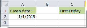
Например, дадена дата 1/1/2015 се намира в клетка A2, както е показано на екранната снимка по-долу. Ако искате да намерите първия петък от месеца въз основа на дадената дата, моля, направете следното.

1. Изберете клетка за показване на резултата. Тук избираме клетка C2.

2. Копирайте и поставете формулата по-долу в него, след което натиснете Въведете ключ.

=CEILING(EOMONTH(A2,-1)-5,7)+6

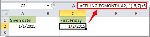
След това датата се показва в клетка C2, това означава, че първият петък на януари 2015 г. е датата 1/2/2015.

бележки:

1. Ако искате да намерите първия петък от други месеци, моля, въведете посочената дата от този месец в клетка A2 и след това използвайте формулата.

2. Във формулата A2 е референтната клетка, която намира дадената дата. Можете да го промените, за да отговаря на вашите нужди.

Намерете последния петък от месеца

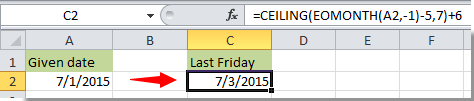
Посочената дата 1/1/2015 се намира в клетка A2, за да намерите последния петък на този месец в Excel, моля, направете следното.

1. Изберете клетка, копирайте формулата по-долу в нея и след това натиснете Въведете ключ за получаване на резултата.

=DATE(YEAR(A2),MONTH(A2)+1,0)+MOD(-WEEKDAY(DATE(YEAR(A2),MONTH(A2)+1,0),2)-2,-7)

Тогава последният петък на януари 2015 г. показва клетка B2.

Забележка: Можете да промените A2 във формулата към референтната клетка на зададената от вас дата.


Още по темата:

Най-добрите инструменти за продуктивност в офиса

🤖 Kutools AI помощник: Революционизирайте анализа на данни въз основа на: Интелигентно изпълнение   |  Генериране на код  |  Създаване на персонализирани формули  |  Анализирайте данни и генерирайте диаграми  |  Извикване на функциите на Kutools...
Популярни функции: Намерете, маркирайте или идентифицирайте дубликати   |  Изтриване на празни редове   |  Комбинирайте колони или клетки без загуба на данни   |   Кръг без формула ...
Супер търсене: VLookup с множество критерии    VLookup с множество стойности  |   VLookup в няколко листа   |   Размито търсене ....
Разширен падащ списък: Бързо създаване на падащ списък   |  Зависим падащ списък   |  Падащ списък с множество избори ....
Мениджър на колони: Добавете конкретен брой колони  |  Преместване на колони  |  Превключване на състоянието на видимост на скритите колони  |  Сравнете диапазони и колони ...
Препоръчани функции: Мрежов фокус   |  Изглед на дизайна   |   Голям формула бар    Мениджър на работни книги и листове   |  Библиотека с ресурси (Автоматичен текст)   |  Избор на дата   |  Комбинирайте работни листове   |  Шифроване/декриптиране на клетки    Изпращайте имейли по списък   |  Супер филтър   |   Специален филтър (филтър получер/курсив/зачертано...) ...
Топ 15 комплекта инструменти12 Текст Инструменти (добавяне на текст, Премахване на символи, ...)   |   50 + Графика Видове (диаграма на Гант, ...)   |   40+ Практичен формули (Изчислете възрастта въз основа на рождения ден, ...)   |   19 вмъкване Инструменти (Въведете QR код, Вмъкване на картина от пътя, ...)   |   12 Конверсия Инструменти (Числа към думи, Валутен обмен, ...)   |   7 Обединяване и разделяне Инструменти (Разширено комбиниране на редове, Разделени клетки, ...)   |   ... и още

Усъвършенствайте уменията си за Excel с Kutools за Excel и изпитайте ефективност, както никога досега. Kutools за Excel предлага над 300 разширени функции за повишаване на производителността и спестяване на време.  Щракнете тук, за да получите функцията, от която се нуждаете най-много...

Описание


Раздел Office Внася интерфейс с раздели в Office и прави работата ви много по-лесна

  • Разрешете редактиране и четене с раздели в Word, Excel, PowerPoint, Publisher, Access, Visio и Project.
  • Отваряйте и създавайте множество документи в нови раздели на един и същ прозорец, а не в нови прозорци.
  • Увеличава вашата производителност с 50% и намалява стотици кликвания на мишката за вас всеки ден!
Comments (12)
Rated 5 out of 5 · 1 ratings
This comment was minimized by the moderator on the site
Even shorter 😅
=lambda(Date;WeekDay;EOMONTH(Date;0)-WEEKDAY(EOMONTH(Date;0);WeekDay+10)+1
Where "WeekDay" parameter is 1=Monday, 7=Sunday
This comment was minimized by the moderator on the site
=lambda(Date;WeekDay;EOMONTH(Date;0)-WEEKDAY(EOMONTH(Date;0);WeekDay+10)+1)

I forgot a bracket at the end
This comment was minimized by the moderator on the site
Vậy công thức tính thứ sáu tuần thứ 2 của tháng như thế nào vậy ban?
This comment was minimized by the moderator on the site
Hi Tâm Cao Điền,
Suppose you want to calculate the second friday of the month based on the given date in A1, you can try the following formula:
=A18-DAY(A18)+CHOOSE(WEEKDAY(A18-DAY(A18),2),11,10,9,8,14,13,12)
This comment was minimized by the moderator on the site
porque cuando lo pruebo tal cual me sale error ?
o sea estoy copiando y pegando y no funciona

alguien sabe?
This comment was minimized by the moderator on the site
Hi andre,
Can you tell me which formula you used in the post? And what error your are experiencing?
This comment was minimized by the moderator on the site
Why not make the "last Friday" formula: =CEILING(EOMONTH(A2,0)-5,7)-1? That works for all dates I have tried....
This comment was minimized by the moderator on the site
Hi Eric,
I hop you are still on this forum and receive my reply.
Thanks so much for an EASY formula. I've never encountered =CEILING.
Rated 5 out of 5
This comment was minimized by the moderator on the site
Hi Eric,
Thanks for sharing it.
This comment was minimized by the moderator on the site
Hello and thank you for this formula. I am not an Excel guru and acnnot easily work out how to change this formula for the last Friday to be the Last Monday, or any other day. Can you please explain how to interpret this.
This comment was minimized by the moderator on the site
Matt,

The way the formula works is: First we find the last day of the month with the EOMONTH() function. For the last day of the current month, we use "0" as the month offset. For the previous month, it would be -1. (Either "=EOMONTH(A2,0)" or "=EOMONTH(A2,-1)".)

Then, in the "=CEILING()" function, we subtract the number of days required to bring us back to Sunday from the day for which we are searching. (For Tuesday, it would be -2, so we make the formula so far: "=CEILING(EOMONTH(A2,0)-2...."

We use the "significance" value of "7" because weeks are seven days long (of course).This finds the date of either the previous Saturday, or the following Saturday (Excel dates started with 1/1/1900, which was a Sunday. So if you enter a "1" in cell A2 with the Long Date format, the cell would read: "Sunday, January 1, 1900".). For that reason, the =CEILING() function, using "7" as the "significance" argument returns Saturday, which is always a multiple of 7 in Excel. Now the formula is "=CEILING(EOMONTH(A2,0)-2,7...".

Now we need to return the date to a Tuesday, so we either subtract 4 for the last Tuesday of the month, or add 3 for the first Tuesday of the next month. So the final formula is, respectively, either "=CEILING(EOMONTH(A2,0)-2,7)-4" or "=CEILING(EOMONTH(A2,0)-2,7)+3".

We can work through the math by assuming the last day of the month is either a Monday (assume its value is 9 - for ease of illustration, so the values do not go negative) or a Wednesday (assume value 11). "EOMONTH()" will return either of those days (9 or 11). Subtracting 2 results in the previous Saturday (value 7) or Monday (value 9), respectively. The CEILING() function then returns, respectively, the previous Saturday (value 7, because the ceiling of 7 with significance 7 is 7) or the current Saturday (value 14, because the ceiling of 9, significance 7, is 14). Subtracting 4 results in the previous Tuesday (value 3) or the current week's Tuesday (value 10), respectively. For the first Tuesday of the following month, adding 3 to the Saturday value (7 or 14) returns either Tuesday value 10, or Tuesday value 17, respectively.


Hopefully that helps you understand so that you can modify the formula as necessary. You can even change it to find the second Tuesday, or second to last Tuesday, by adding or subtracting an additional 7, respectively.
This comment was minimized by the moderator on the site
Hi Matt,
You just need to change the last number -7 to -1 to solove the problem.
=DATE(YEAR(A2),MONTH(A2)+1,0)+MOD(-WEEKDAY(DATE(YEAR(A2),MONTH(A2)+1,0),2)-2,-1)
There are no comments posted here yet
Please leave your comments in English
Posting as Guest
×
Rate this post:
0   Characters
Suggested Locations