Прескочи на основното съдържание

Как да върна множество съвпадащи стойности въз основа на един или множество критерии в Excel?

Автор: Xiaoyang Последна промяна: 2022-07-28

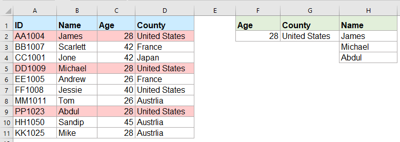
Обикновено търсенето на конкретна стойност и връщането на съответстващия елемент е лесно за повечето от нас с помощта на функцията VLOOKUP. Но опитвали ли сте някога да върнете множество съответстващи стойности въз основа на един или повече критерии, както е показано на следната екранна снимка? В тази статия ще представя някои формули за решаване на тази сложна задача в Excel.

Връща множество съвпадащи стойности въз основа на един или множество критерии с формули за масиви


Връща множество съвпадащи стойности въз основа на един или множество критерии с формули за масиви

Например, искам да извлека всички имена, чиято възраст е 28 и идват от Съединените щати, моля, приложете следната формула:

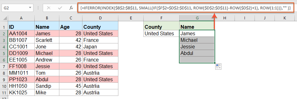
1. Копирайте или въведете формулата по-долу в празна клетка, където искате да намерите резултата:

=INDEX($B$2:$B$11, SMALL(IF(COUNTIF($F$2, $C$2:$C$11)*COUNTIF($G$2, $D$2:$D$11), ROW($A$2:$D$11)-MIN(ROW($A$2:$D$11))+1), ROW(A1)), COLUMN(A1))

Забележка: В горната формула, B2: B11 е колоната, от която се връща съответстващата стойност; F2, C2:C11 са първото условие и данните в колоната, която съдържа първото условие; G2, D2: D11 са второто условие и данните в колоната, които съдържат това условие, моля, променете ги според вашите нужди.

2. След това натиснете Ctrl + Shift + Enter клавиши, за да получите първия съответстващ резултат, след което изберете първата клетка с формула и плъзнете манипулатора за попълване надолу към клетките, докато се покаже стойността на грешката, сега всички съответстващи стойности се връщат, както е показано на екранната снимка по-долу:

Съвети: Ако просто трябва да върнете всички съответстващи стойности въз основа на едно условие, моля, приложете формулата за масив по-долу:

=IFERROR(INDEX($B$2:$B$11, SMALL(IF($F$2=$D$2:$D$11, ROW($D$2:$D$11)-ROW($D$2)+1), ROW(1:1))),"" )


Още относителни статии:

  • Връщане на множество стойности за търсене в една клетка, разделена със запетая
  • В Excel можем да приложим функцията VLOOKUP, за да върнем първата съвпадаща стойност от клетки на таблица, но понякога трябва да извлечем всички съвпадащи стойности и след това да ги разделим със специфичен разделител, като запетая, тире и т.н., в една клетка, както е показано на следната екранна снимка. Как можем да получим и върнем множество стойности за търсене в една клетка, разделена със запетая, в Excel?
  • Vlookup и връщане на няколко съвпадащи стойности наведнъж в Google Sheet
  • Нормалната функция Vlookup в Google sheet може да ви помогне да намерите и върнете първата съответстваща стойност въз основа на дадени данни. Но понякога може да се наложи да направите vlookup и да върнете всички съответстващи стойности, както е показано на следната екранна снимка. Имате ли добри и лесни начини за решаване на тази задача в Google лист?
  • Vlookup и връщане на множество стойности от падащия списък
  • В Excel, как бихте могли да направите vlooking и да върнете множество съответни стойности от падащ списък, което означава, че когато изберете един елемент от падащия списък, всичките му относителни стойности се показват наведнъж, както е показано на следната екранна снимка. В тази статия ще представя решението стъпка по стъпка.
  • Vlookup и връщане на множество стойности вертикално в Excel
  • Обикновено можете да използвате функцията Vlookup, за да получите първата съответстваща стойност, но понякога искате да върнете всички съответстващи записи въз основа на конкретен критерий. В тази статия ще говоря за това как да направя vlookup и да върна всички съвпадащи стойности вертикално, хоризонтално или в една клетка.
  • Vlookup и връщане на съвпадащи данни между две стойности в Excel
  • В Excel можем да приложим нормалната функция Vlookup, за да получим съответната стойност въз основа на дадени данни. Но понякога искаме да направим vlookup и да върнем съвпадащата стойност между две стойности, както е показано на следната екранна снимка, как бихте могли да се справите с тази задача в Excel?


  • Супер Формула Бар (лесно редактиране на няколко реда текст и формула); Оформление за четене (лесно четене и редактиране на голям брой клетки); Поставяне във филтриран диапазон...
  • Обединяване на клетки/редове/колони и съхраняване на данни; Съдържание на разделени клетки; Комбинирайте дублиращи се редове и сума/средно... Предотвратяване на дублиращи се клетки; Сравнете диапазони...
  • Изберете Дублиран или Уникален редове; Изберете Празни редове (всички клетки са празни); Super Find и Fuzzy Find в много работни тетрадки; Произволен избор...
  • Точно копие Множество клетки без промяна на референтната формула; Автоматично създаване на препратки към множество листа; Вмъкване на куршуми, квадратчета за отметка и други...
  • Любими и бързо вмъкнати формули, диапазони, диаграми и снимки; Шифроване на клетки с парола; Създаване на пощенски списък и изпращайте имейли...
  • Извличане на текст, Добавяне на текст, Премахване по позиция, Премахване на пространството; Създаване и отпечатване на междинни суми за пейджинг; Конвертиране на съдържание и коментари между клетки...
  • Супер филтър (запазване и прилагане на филтърни схеми към други листове); Разширено сортиране по месец/седмица/ден, честота и други; Специален филтър с удебелен шрифт, курсив...
  • Комбинирайте работни тетрадки и работни листове; Обединяване на таблици въз основа на ключови колони; Разделете данните на няколко листа; Пакетно конвертиране на xls, xlsx и PDF...
  • Групиране на обобщена таблица по номер на седмицата, ден от седмицата и други... Показване на отключени, заключени клетки с различни цветове; Маркирайте клетки, които имат формула/име...
kte tab 201905
  • Разрешете редактиране и четене с раздели в Word, Excel, PowerPoint, Publisher, Access, Visio и Project.
  • Отваряйте и създавайте множество документи в нови раздели на един и същ прозорец, а не в нови прозорци.
  • Увеличава вашата производителност с 50% и намалява стотици кликвания на мишката за вас всеки ден!
officetab отдолу


Comments (25)
No ratings yet. Be the first to rate!
This comment was minimized by the moderator on the site
Hi, if there are duplicate values (e.g. two adams), how do i make sure that it only returns 1 adam and not 2?
This comment was minimized by the moderator on the site
Hello, Bobby,
To extract only unique matching values, you should apply the below formula:
After pasting the formula, please press Ctrl + Shift + Enter keys together to get the correct result.
=IFERROR(INDEX($B$2:$B$5, MATCH(0, COUNTIF(H1:$H$1, $B$2:$B$5)+IF($D$2:$D$5<>$G$2, 1, 0)+IF($C$2:$C$5<>$F$2, 1, 0), 0)), "")

Please have a try, hope it can help you!
This comment was minimized by the moderator on the site
Hi,

Thanks for posting these examples.
I'm trying to implement this in my own sheet, but don't get it to work (maybe because I'm using an europe version of excel)?

I want to get the dates of the days that I had my shifts or that I have worked 'some' (>0) hours for a client.

So in I3 is the name and in J3 the month. K3 and L3 are the shifts (1 is worked) and hours (don't know how to set this, should be more than zero)

My expected results are in:
Shifts: I7 and I8
hours: J7

So I worked more than 0 hours for 'person 2' in oktober on 3-10-2022
had shifts for person 2 on '10-10-2022' and 28-10-2022

When I add '=INDEX($B$2:$B$11, SMALL(IF(COUNTIF($F$2, $C$2:$C$11)*COUNTIF($G$2, $D$2:$D$11), ROW($A$2:$D$11)-MIN(ROW($A$2:$D$11))+1), ROW(A1)), COLUMN(A1))' in my excel sheet, it doesn't allow the comma between the different parts of the formula.
So I need to change them to ';'.
But when I try it it always says: '#NAME?'

So can someone help me with this?

Kind regards,

Bas
[img]https://drive.google.com/file/d/1iIPQKuj_PNhqWyWlwJ4IQTqGNEd6B9Hw/view?usp=share_link[/img]
This comment was minimized by the moderator on the site
Hi,

First, thank you for sharing!

Can you please provide a solution to the case below:

I have 3 columns (A: Containing reference information, B: Containing information to be searched, C: Search result)

Image url is provided below

https://ibb.co/VHCd09K

Column A-------------------------Column B------------Column C
File Name-------------------------Name----------------File Name, Document Name, Element Name, Name
Changed Element-----------------Element--------------Changed Element, Element Name, Element ID
Column Location
Document Name
Element Name
Name
Category
Warranty
Slope
Element ID

What I need is to search in column A for any partial match with cell B2 (Name) or B3 (Element) and get the result in one cell,

Thank you, Behzad
This comment was minimized by the moderator on the site
Hello, Behzad
Maybe the below User Defined Function can help you.
Public Function ConcatPartLookUp(rngInput As Range, rngSource As Range, Optional strDelimiter As String, Optional blCaseSensitive)
Dim rng As Range
If strDelimiter = "" Then strDelimiter = ","
If IsMissing(blCaseSensitive) Then
    blCaseSensitive = False
Else
    blCaseSensitive = True
End If
For Each rng In rngSource
    If blCaseSensitive Then
        If InStr(1, rng.Value, rngInput.Value, vbBinaryCompare) > 0 Then ConcatPartLookUp = ConcatPartLookUp & strDelimiter & rng.Value
    Else
        If InStr(1, rng.Value, rngInput.Value, vbTextCompare) > 0 Then ConcatPartLookUp = ConcatPartLookUp & strDelimiter & rng.Value
    End If
Next
If Len(ConcatPartLookUp) > 0 Then ConcatPartLookUp = Mid(ConcatPartLookUp, 2, Len(ConcatPartLookUp))
End Function


After copying and pasting this code, and then use this formula:=ConcatPartLookUp(B2,$A$2:$A$8) to get the result you need.
Please have a try, hope it can help you!
This comment was minimized by the moderator on the site
Heyi, thank you for the formula. It worked for "fixed" values / text as criterias. However, one of the criterias i'm trying to use is a condition (values <>0 ), but does not work the described formula. Do you guys know what should i change to adapt the formula so I can have a condition as one of the criterias, please?

Best,

João
This comment was minimized by the moderator on the site
Hello, Marcus
To solve your problem, please view this article:
https://www.extendoffice.com/documents/excel/6393-excel-vlookup-function.html#b3-2
There are some detailed explanations of this task. You just need to change the criteira to your own.
Thank you!
This comment was minimized by the moderator on the site
Hi,

if in cell H1 i write "Name" and wanted to link that with the formula, how would that work?
Then I could write "ID" in cell H1 and would automatically get as a result: AA1004; DD1009; PP1023 (for the first formula)

Thank you in advance!
This comment was minimized by the moderator on the site
Hello, Marie
Sorry, i can't get the point of your first problem, could you explain your problem more clearly and detailedly? Or you can insert a screenshot here to describe your problem.
As for the second question, you just need to change the cell reference as this:
=INDEX($A$2:$A$11, SMALL(IF(COUNTIF($F$2, $C$2:$C$11)*COUNTIF($G$2, $D$2:$D$11), ROW($A$2:$D$11)-MIN(ROW($A$2:$D$11))+1), ROW(A1)), COLUMN(A1))

Remeber to press Ctrl + Shift + Enter keys together.
Please try, hope it can help you!
This comment was minimized by the moderator on the site
Hello,
what would be needed to expand the first formula in the following case:
Some IDs are Blank (e.g. cell A5 is blank) and I would like an additional condition outputting lines only when the IDs are not blank. (So the output should then be James and Abdul.
Thanks!
This comment was minimized by the moderator on the site
Hello, Jo,
To solve your problem, please apply the below formula:
=INDEX($B$2:$B$11, SMALL(IF(COUNTIF($F$2, $C$2:$C$11)*COUNTIF($G$2, $D$2:$D$11)*($A$2:$A$11<>0), ROW($A$2:$D$11)-MIN(ROW($A$2:$D$11))+1), ROW(A1)), COLUMN(A1))

Please have a ry, hope it can help you!
This comment was minimized by the moderator on the site
hello,
ive tried using the formula and it either generates a value of 0 or the image attached
This comment was minimized by the moderator on the site
Hello, Milku
Your screenshot showed WPS software of MAC version, so I am not sure whether our formula is available.
I uploaded an Excel file to here, you can try to see if it can calculate correctly in you environment.
Thank you!
This comment was minimized by the moderator on the site
When I use the second formula and drag down, nothing appears. The formula result (fx) says it should be returning something but it is blank. How do I correct this?
This comment was minimized by the moderator on the site
Hello Alysia,

Glad to help. I tried the second formula in the article and drag the formula down, the rest of results were returned. I think there may be two reasons for your problem. First, maybe you forget to press Ctrl + Shift + Enter keys to enter the formula. Second, the matching result is only one, so no other results are not returned. Please have a check.

Sincerely,
Mandy
This comment was minimized by the moderator on the site
Hi,

I was wondering if it at all possible to enter a 2nd criteria but from the same range as the 1st criteria,

For example with the used example above i would like to search for the names of people from both America and France So cell F3 would have France, Scarlett & Andrew would also populate in the list in Column G

Thank you for assistance in advance.
This comment was minimized by the moderator on the site
Hello Nick,

Glad to help. If you want to get the names of people from both America and France, I advise you to use our formula twice to get the result. Please see the screenshot, In F2 and G2 are values "United States" and "France". Apply formula =IFERROR(INDEX($B$2:$B$11, SMALL(IF($F$2=$D$2:$D$11, ROW($D$2:$D$11)-ROW($D$2)+1), ROW(1:1))),"" ) to get the results for America. And apply formula =IFERROR(INDEX($B$2:$B$11, SMALL(IF($G$2=$D$2:$D$11, ROW($D$2:$D$11)-ROW($D$2)+1), ROW(1:1))),"" ) to get the results for France. It's simple. Please have a try.

Sincerely,
Mandy
This comment was minimized by the moderator on the site
In the first example, what change to the formula would be needed to return everyone who was less than 28 years old?
There are no comments posted here yet
Load More
Please leave your comments in English
Posting as Guest
×
Rate this post:
0   Characters
Suggested Locations